2. 3D reconstruction of MERFISH mouse hypothalamic preoptic region
Then, we perform the de novo 3D construction of MERFISH mouse hypothalamic preoptic region using STAIR. STAIR first learn and integrate spatial feature of slices using STAIR-Emb, defing inter-slice semantic distances based on the slice-level attention scores. Then, STAIR utilize a minimum spanning tree (MST) based on these distances to reconstruct the z-axis coordinates. Finally, the reconstructed z-coordinates guide STAIR-Loc to align the x- and y- axes.
[1]:
import warnings
warnings.filterwarnings("ignore")

import numpy as np
import pandas as pd
import anndata as ad
import scanpy as sc
import matplotlib.pyplot as plt

from STAIR.emb_alignment import Emb_Align
from STAIR.utils import *
Load data
[2]:
adata = sc.read('./data/hypothalamic_preoptic.h5ad')
adata
[2]:
AnnData object with n_obs × n_vars = 64373 × 155
    obs: 'Animal_ID', 'Animal_sex', 'Behavior', 'Bregma', 'Centroid_X', 'Centroid_Y', 'Cell_class', 'Neuron_cluster_ID', 'slices', 'Coord_X', 'Coord_Y', 'x', 'y', 'z', 'cell_type', 'batch', 'n_genes'
    var: 'n_cells'
    uns: 'batch_colors'
    obsm: 'spatial', 'spatial_2d_raw', 'spatial_2d_raw_rotate', 'spatial_2d_μm', 'spatial_2d_μm_rotate', 'spatial_3d', 'spatial_3d_raw', 'spatial_3d_raw_rotate', 'spatial_3d_μm', 'spatial_3d_μm_rotate'
    layers: 'noise1', 'noise2', 'noise3', 'noise4'
We visualize the cell types and 3D coordinates provided in the original research.
[3]:
from matplotlib.pyplot import rc_context
with rc_context({'figure.figsize': (5,5)}):
    sc.pl.embedding(
                    adata,
                    basis="spatial_3d_μm",
                    na_color=(1, 1, 1, 0),
                    projection="3d",
                    s=0.1,
                    color="cell_type",
                    title='Ground truth 3D coordinates'
                )

To test the spatial construction capability of STAIR, we randomly rotate and translate the x- and y- axes of the second and subsequent slices.
[4]:
# rotate & translate

# import math
# def rotate(angle,valuex,valuey):
#     rotatex = math.cos(angle)*valuex -math.sin(angle)*valuey
#     rotatey = math.cos(angle)*valuey + math.sin(angle)* valuex
#     return np.hstack((rotatex[:,None], rotatey[:,None]))


# slices = sorted(list(set(adata_all.obs['z'])))

# adata_raw_list = [adata_all[adata_all.obs['z']==slice].copy() for slice in slices]

# angles = np.random.uniform(0,2*np.pi,len(slices)-1)
# tran_xs = np.random.uniform(-1800,1800,len(slices)-1)
# tran_ys = np.random.uniform(-1800,1800,len(slices)-1)
# pd.DataFrame(np.vstack((angles, tran_xs, tran_ys)).T, columns=['angle', 'tran_x', 'tran_y']).to_csv('trans_gt.csv')


# adata_raw_rotate_list = []

# for i in range(len(slices)):
#     slice_tmp = slices[i]
#     adata_raw_tmp = adata_raw_list[i]

#     if i !=0:
#         angle_tmp = angles[i-1]
#         tran_x_tmp = tran_xs[i-1]
#         tran_y_tmp = tran_ys[i-1]
#         adata_raw_tmp.obsm['spatial_2d_raw_rotate'] = rotate(angle_tmp,adata_raw_tmp.obsm['spatial_2d_raw'][:,0],adata_raw_tmp.obsm['spatial_2d_raw'][:,1])
#         adata_raw_tmp.obsm['spatial_2d_raw_rotate'] = np.vstack((adata_raw_tmp.obsm['spatial_2d_raw_rotate'][:,0] + tran_x_tmp,
#                                                                  adata_raw_tmp.obsm['spatial_2d_raw_rotate'][:,1] + tran_y_tmp)).T
#         adata_raw_tmp.obsm['spatial_3d_raw_rotate'] = np.hstack((adata_raw_tmp.obsm['spatial_2d_raw_rotate'], adata_raw_tmp.obsm['spatial_3d_raw'][:,2][:,None]))

#         adata_raw_tmp.obsm['spatial_2d_μm_rotate'] = rotate(angle_tmp,adata_raw_tmp.obsm['spatial_2d_μm'][:,0],adata_raw_tmp.obsm['spatial_2d_μm'][:,1])
#         adata_raw_tmp.obsm['spatial_2d_μm_rotate'] = np.vstack((adata_raw_tmp.obsm['spatial_2d_μm_rotate'][:,0] + tran_x_tmp,
#                                                                  adata_raw_tmp.obsm['spatial_2d_μm_rotate'][:,1] + tran_y_tmp)).T
#         adata_raw_tmp.obsm['spatial_3d_μm_rotate'] = np.hstack((adata_raw_tmp.obsm['spatial_2d_μm_rotate'], adata_raw_tmp.obsm['spatial_3d_μm'][:,2][:,None]))
#     else:
#         adata_raw_tmp.obsm['spatial_2d_raw_rotate'] = adata_raw_tmp.obsm['spatial_2d_raw']
#         adata_raw_tmp.obsm['spatial_3d_raw_rotate'] = adata_raw_tmp.obsm['spatial_3d_raw']
#         adata_raw_tmp.obsm['spatial_2d_μm_rotate'] = adata_raw_tmp.obsm['spatial_2d_μm']
#         adata_raw_tmp.obsm['spatial_3d_μm_rotate'] = adata_raw_tmp.obsm['spatial_3d_μm']

#     adata_raw_rotate_list.append(adata_raw_tmp)

# adata = ad.concat(adata_rotate_list)
# adata.write('./data/hypothalamic_preoptic.h5ad')

# Visualize
fig, axs = plt.subplots(1, 2, figsize=(8,3.2),constrained_layout=True)

[axs[i].axis('off') for i in range(2)]
axs[0].set_xlim([adata.obsm['spatial'].min(0)[0], adata.obsm['spatial'].max(0)[0]])
axs[0].set_ylim([adata.obsm['spatial'].min(0)[1], adata.obsm['spatial'].max(0)[1]])
axs[1].set_xlim([adata.obsm['spatial_2d_μm_rotate'].min(0)[0], adata.obsm['spatial_2d_μm_rotate'].max(0)[0]])
axs[1].set_ylim([adata.obsm['spatial_2d_μm_rotate'].min(0)[1], adata.obsm['spatial_2d_μm_rotate'].max(0)[1]])

sc.pl.embedding(adata, basis='spatial', color='batch', title='Ground truth 2D coordinates', frameon=False, s=20, show=False, ax=axs[0])
sc.pl.embedding(adata, basis='spatial_2d_μm_rotate', color='batch', title='Rotated 2D coordinates', frameon=False, s=20, show=False, ax=axs[1])

plt.show()
plt.close()

Preprocess
[5]:
result_path = construct_folder('hypothalamic')
keys_use = ['A0', 'A1', 'A2', 'A3', 'A4', 'A5', 'A6', 'A7', 'A8', 'A9', 'A10', 'A11']
[6]:
# Construct the model
emb_align = Emb_Align(adata, batch_key='batch', result_path=result_path)
emb_align.prepare()

# Preprocessing
emb_align.preprocess()
emb_align.latent()
100%|████████████████████████████████████████████████████████████████████████| 100/100 [11:19<00:00, 6.80s/it]
Spatial embedding alignment
First, we align the spatial embeddings of these slices, which facilitates subsequent spatial reconstruction
[7]:
# Construct the heterogeneous graph
emb_align.prepare_hgat( spatial_key = 'spatial_2d_μm_rotate',
                        slice_order = keys_use)

# learning & integrating
emb_align.train_hgat()
adata, atte = emb_align.predict_hgat()
atte.to_csv(f'{result_path}/embedding/attention.csv')

# clustering of spatial embedding
adata = cluster_func(adata, clustering='mclust', use_rep='STAIR', cluster_num=13, key_add='STAIR')
100%|████████████████████████████████████████████████████████████████████████| 150/150 [00:54<00:00,  2.76it/s]
R[write to console]:                    __           __
   ____ ___  _____/ /_  _______/ /_
  / __ `__ \/ ___/ / / / / ___/ __/
 / / / / / / /__/ / /_/ (__  ) /_
/_/ /_/ /_/\___/_/\__,_/____/\__/   version 6.0.0
Type 'citation("mclust")' for citing this R package in publications.
fitting ...
  |======================================================================| 100%
[8]:
# Visualization

sc.pp.neighbors(adata, use_rep='STAIR')
sc.tl.umap(adata, min_dist=0.2)

from matplotlib.pyplot import rc_context
with rc_context({'figure.figsize': (4,4)}):
    sc.pl.umap(adata, color=['batch', 'STAIR'], frameon=False, ncols=3, show=True)

[9]:
# annotation
adata.obs['Domain'] = adata.obs['STAIR'].replace({ '1.0': 'stHY', '10.0': 'VLPO', '11.0': '3V', '12.0': 'BAC', '13.0': 'PVN', '2.0': 'MnPO',
                                                   '3.0': 'Hypo', '4.0': 'Pe', '5.0': 'MPA', '6.0': 'opn', '7.0': 'MPN', '8.0': 'BNST', '9.0': 'ACA_Fx'}
                                                )

adata.obs['Domain'] = adata.obs['Domain'].astype('category').cat.set_categories(['stHY', 'MnPO', 'Hypo', 'Pe', 'MPA', 'opn', 'MPN', 'BNST', 'ACA_Fx', 'VLPO', '3V', 'BAC', 'PVN'])

import matplotlib
hex_colors = [plt.matplotlib.colors.rgb2hex(color) for color in plt.cm.tab20.colors]
domains = adata.obs['Domain'].cat.categories.tolist()
adata.uns['Domain_colors'] = hex_colors[:len(set(adata.obs['Domain']))]

with rc_context({'figure.figsize': (4,4)}):
    sc.pl.umap(adata, color=['Domain'], frameon=False, ncols=3, show=True)

[10]:
# 2D visualization of spatial domain

n_row = 3
n_col = 4
fig, axs = plt.subplots(n_row, n_col, figsize=(9.5,7.8),constrained_layout=True)

index = 0
for i in range(n_row):
    for j in range(n_col):
        axs[i,j].get_xaxis().set_visible(False)
        axs[i,j].get_yaxis().set_visible(False)
        axs[i,j].axis('off')
        axs[i,j].set_xlim([adata.obsm['spatial'].min(0)[0], adata.obsm['spatial'].max(0)[0]])
        axs[i,j].set_ylim([adata.obsm['spatial'].min(0)[1], adata.obsm['spatial'].max(0)[1]])
        if index < len(keys_use):
            key = keys_use[index]
            adata_tmp = adata[adata.obs['batch']==key].copy()
            if j<(n_col-1):
                sc.pl.embedding(adata_tmp, basis='spatial', color='Domain', title=key, frameon=False, legend_loc='right', s=30, show=False, ax=axs[i,j])
                j += 1
            else:
                sc.pl.embedding(adata_tmp, basis='spatial', color='Domain', title=key, frameon=False, s=30, show=False, ax=axs[i,j])
                i += 1
                j = 0

        index += 1
plt.show()
plt.close()
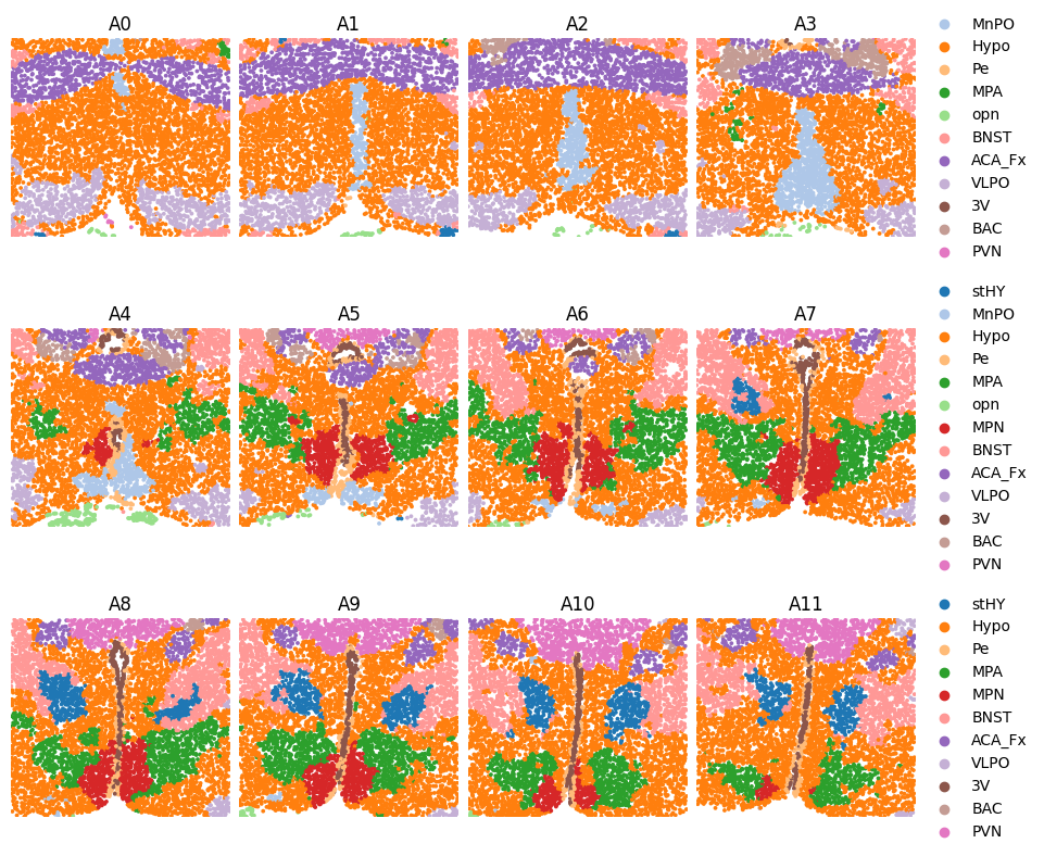
Reconstruction in z-axis
Next, we focus on the z-axis reconstruction based on slice level attention in the STAIR-Emb module. We visualize the inter-slice attention scores using heatmap.
[11]:
import seaborn as sns
vmax = atte[atte!=1].max().max()
vmin = atte[atte!=1].min().min()
plt.figure(figsize=(4.4,4))
sns.heatmap(atte, vmax=vmax, vmin=vmin)
plt.show()
plt.close()

There are higher attention scores between physically closer slices. We quantify the correlation between attention scores and spatial distances.
[12]:
# attention-spatial consistency

from scipy.stats import spearmanr

use = adata.obs[['batch', 'Bregma']].drop_duplicates()
use.index = use['batch']
use = use['Bregma']

attes = []
dists = []
for i in keys_use:
    for j in keys_use:
        if (i != j) & (i < j):
            atte_tmp = (atte.loc[i,j] + atte.loc[j,i]) / 2
            dist_tmp = abs(use[i] - use[j])
            attes.append(atte_tmp)
            dists.append(dist_tmp)


plt.figure(figsize=(3,3))
plt.scatter(dists, attes, s=5)
plt.xlabel('Bregma distance', fontsize=13)
plt.ylabel('Attention score', fontsize=13)
plt.text(0.28, 0.115, 'Spearman: ' + str(round(spearmanr(attes, dists)[0], 2)))
plt.show()
plt.close()

The strong correlation prompts us to reconstruct the z-axis coordinates according to attention scores.
[13]:
from STAIR.loc_prediction import sort_slices
dists = sort_slices(atte, start='A11')
dists
[13]:
{'A11': 0.0,
 'A10': 0.885701893,
 'A9': 1.770533613,
 'A8': 2.6595647380000003,
 'A7': 3.5472318000000005,
 'A6': 4.436391565000001,
 'A5': 5.322045235000001,
 'A4': 6.213104990000001,
 'A3': 7.103802040000001,
 'A2': 7.985913619000001,
 'A1': 8.867480269000001,
 'A0': 9.754753862000001}
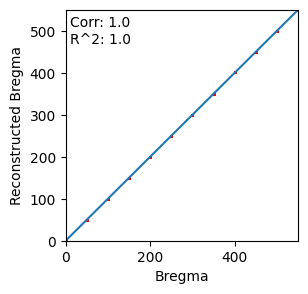
[14]:
import scanpy as sc
import numpy as np

adata.obs['z_rec'] = adata.obs['batch'].replace(dists).astype(float)
adata.obs['z_rec'] = (adata.obs['z_rec']- adata.obs['z_rec'].min()) / (adata.obs['z_rec'].max() - adata.obs['z_rec'].min())
adata.obs['z_rec']

z_max, z_min = adata.obs['z'].max(), adata.obs['z'].min()
adata.obs['z_rec'] = adata.obs['z_rec'] * (z_max - z_min) + z_min
adata.obs['z_rec']

from scipy.stats import pearsonr
from sklearn.metrics import r2_score
import matplotlib.pyplot as plt
import numpy as np

vmin = np.array(adata.obs['z_rec'].tolist() + adata.obs['z'].tolist()).min()
vmax = np.array(adata.obs['z_rec'].tolist() + adata.obs['z'].tolist()).max()

plt.figure(figsize=(3,3))
plt.plot([vmin, vmax],[vmin, vmax])
plt.scatter(adata.obs['z'], adata.obs['z_rec'], s=1, c='r')
plt.text(10,470,'Corr: ' + str(pearsonr(adata.obs['z'], adata.obs['z_rec'])[0].round(2)) + '\n' + \
         "R^2: " + str(r2_score(adata.obs['z'], adata.obs['z_rec']).round(2))
         )
plt.xlim([vmin, vmax])
plt.ylim([vmin, vmax])
plt.xlabel('Bregma')
plt.ylabel('Reconstructed Bregma')
plt.show()
plt.close()
Spatial location alignment in x-axis and y-axis
Finally, STAIR-Loc aligns the x- and y- axes of slices based on the reconstructed z-coordinates.
[15]:
adata.obs[['batch', 'z_rec']].drop_duplicates().sort_values('z_rec', ascending=False)['batch'].tolist()
[15]:
['A0', 'A1', 'A2', 'A3', 'A4', 'A5', 'A6', 'A7', 'A8', 'A9', 'A10', 'A11']
[16]:
from STAIR.loc_alignment import Loc_Align

keys_order = adata.obs[['batch', 'z_rec']].drop_duplicates().sort_values('z_rec', ascending=False)['batch'].tolist()
loc_align = Loc_Align(adata, batch_key='batch', batch_order=keys_order, result_path=result_path)

loc_align.init_align(   emb_key = 'STAIR',
                        spatial_key = 'spatial_2d_μm_rotate',
                        num_mnn = 1  )

loc_align.detect_fine_points(  domain_key = 'Domain',
                               slice_boundary = True,
                               domain_boundary = True,
                               num_domains = 1,
                               alpha = 70,
                               return_result = False)

loc_align.plot_edge(spatial_key = 'transform_init',
                    figsize = (6,6),
                    s=2)

adata = loc_align.fine_align()

# import pandas as pd
# transform_fine = pd.DataFrame(adata.obsm['transform_fine'], index=adata.obs_names, columns=['x', 'y'])
# transform_init = pd.DataFrame(adata.obsm['transform_init'], index=adata.obs_names, columns=['x', 'y'])
# transform_fine.to_csv(f'{result_path}/location/transform_fine.csv')
# transform_init.to_csv(f'{result_path}/location/transform_init.csv')
Performing initial alignment of the 1 pair of data...
Finding similar pairs using STAIR...
Aligning slices using 645 pairs of similar spots!
Performing initial alignment of the 2 pair of data...
Finding similar pairs using STAIR...
Aligning slices using 662 pairs of similar spots!
Performing initial alignment of the 3 pair of data...
Finding similar pairs using STAIR...
Aligning slices using 560 pairs of similar spots!
Performing initial alignment of the 4 pair of data...
Finding similar pairs using STAIR...
Aligning slices using 585 pairs of similar spots!
Performing initial alignment of the 5 pair of data...
Finding similar pairs using STAIR...
Aligning slices using 635 pairs of similar spots!
Performing initial alignment of the 6 pair of data...
Finding similar pairs using STAIR...
Aligning slices using 695 pairs of similar spots!
Performing initial alignment of the 7 pair of data...
Finding similar pairs using STAIR...
Aligning slices using 672 pairs of similar spots!
Performing initial alignment of the 8 pair of data...
Finding similar pairs using STAIR...
Aligning slices using 756 pairs of similar spots!
Performing initial alignment of the 9 pair of data...
Finding similar pairs using STAIR...
Aligning slices using 684 pairs of similar spots!
Performing initial alignment of the 10 pair of data...
Finding similar pairs using STAIR...
Aligning slices using 724 pairs of similar spots!
Performing initial alignment of the 11 pair of data...
Finding similar pairs using STAIR...
Aligning slices using 754 pairs of similar spots!
Performing fine alignment of the 1 pair of data...
Performing fine alignment of the 2 pair of data...
Performing fine alignment of the 3 pair of data...
Performing fine alignment of the 4 pair of data...
Performing fine alignment of the 5 pair of data...
Performing fine alignment of the 6 pair of data...
Performing fine alignment of the 7 pair of data...
Performing fine alignment of the 8 pair of data...
Performing fine alignment of the 9 pair of data...
Performing fine alignment of the 10 pair of data...
Performing fine alignment of the 11 pair of data...
[17]:
adata.obs['Domain'] = adata.obs['Domain'].astype('category').cat.set_categories(['stHY', 'MnPO', 'Hypo', 'Pe', 'MPA', 'opn', 'MPN', 'BNST', 'ACA_Fx', 'VLPO', '3V', 'BAC', 'PVN'])
adata.uns['Domain_colors'] = hex_colors[:len(set(adata.obs['Domain']))]

## initial alignment
with rc_context({'figure.figsize': (3,3)}):
    sc.pl.embedding(adata, basis='transform_init', color=['batch', 'Domain'],
                    frameon=False, ncols=2, show=True, s=15)

## fine alignment
with rc_context({'figure.figsize': (3,3)}):
    sc.pl.embedding(adata, basis='transform_fine', color=['batch', 'Domain'],
                    frameon=False, ncols=2, show=True, s=15)


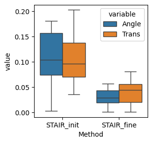
We evaluate the accuracy of positional alignment quantitatively.
[18]:
from STAIR.location.transformation import best_fit_transform

import math
def cacul_angle(cos_val, sin_val):
    tan_val = math.sqrt(1 - cos_val**2) / cos_val  # 利用三角恒等式求解正切值
    if cos_val > 0:
        if sin_val >= 0:
            theta = math.atan(tan_val)  # 计算角度,注意使用math.atan函数
        else:
            theta = 2*math.pi - math.atan(tan_val)
    else:
        if sin_val >= 0:
            theta = math.pi - math.atan(tan_val)
        else:
            theta = math.pi + math.atan(tan_val)
    return theta


angle_inits = []
angle_fines = []
trans_inits = []
trans_fines = []
for key in keys_use[1:]:
    init = best_fit_transform(adata[adata.obs['batch']==key].obsm['transform_init'], adata[adata.obs['batch']==key].obsm['spatial_2d_μm'])[1:]
    fine = best_fit_transform(adata[adata.obs['batch']==key].obsm['transform_fine'], adata[adata.obs['batch']==key].obsm['spatial_2d_μm'])[1:]
    angle_inits.append(cacul_angle(cos_val=init[0][0,0], sin_val=init[0][0,0]))
    angle_fines.append(cacul_angle(cos_val=fine[0][0,0], sin_val=fine[0][0,0]))
    trans_inits.append(np.array(init[1]))
    trans_fines.append(np.array(fine[1]))

error_init = pd.DataFrame(np.array(trans_inits), index=keys_use[1:], columns=['trans_x', 'trans_y'])
error_fine = pd.DataFrame(np.array(trans_fines), index=keys_use[1:], columns=['trans_x', 'trans_y'])
error_init['Angle'] = angle_inits
error_init['Method'] = 'STAIR_init'
error_fine['Angle'] = angle_fines
error_fine['Method'] = 'STAIR_fine'
error = pd.concat([error_init, error_fine])

def square(x):
    return (x ** 2)

error['Trans'] = np.sqrt(error['trans_x'].map(square) + error['trans_y'].map(square))/1000
error = error.iloc[:,2:]

error.melt(id_vars=['Method'])

plt.figure(figsize=(3,3))
sns.boxplot(x='Method', y='value', hue='variable', data=error.melt(id_vars=['Method']))
plt.show()
plt.close()
3D Visualization
[19]:
# 3D

adata.obsm['rec_3d'] = adata.obs[['x_aligned', 'y_aligned', 'z_rec']].values

with rc_context({'figure.figsize': (5,5)}):
    sc.pl.embedding(
                    adata,
                    basis="rec_3d",
                    na_color=(1, 1, 1, 0),
                    projection="3d",
                    color="Domain",
                    title='De novo reconstructed 3D coordinates'
                   )

[20]:
with rc_context({'figure.figsize': (5,5)}):
    sc.pl.embedding(
                    adata,
                    basis="spatial_3d_μm",
                    na_color=(1, 1, 1, 0),
                    projection="3d",
                    color="Domain",
                    title='Ground truth 3D coordinates'
                )

Save
[21]:
adata.write(f'{result_path}/adata.h5ad')