3. 3D reconstruction of ST mouse brain

Next, we use the same steps as in the previous section to perform de novo 3D reconstruction of the ST mouse brain.

import warnings
warnings.filterwarnings("ignore")

import numpy as np
import pandas as pd
import anndata as ad
import scanpy as sc
import matplotlib.pyplot as plt

from STAIR.emb_alignment import Emb_Align
from STAIR.loc_alignment import Loc_Align
from STAIR.loc_prediction import sort_slices
from STAIR.loc_prediction import loc_predict_z
from STAIR.utils import *

Load data

adata = sc.read('./data/st_brain.h5ad')

result_path = construct_folder('st_brain')

keys_use = ['01A', '02A', '03A', '04A', '05A', '06A', '07A', '08A',
            '09A', '10B', '11A', '12A', '13A', '14A', '15B', '16A',
            '17A', '18A', '19A', '20B', '21A', '22A', '23A', '24A',
            '25A', '26B', '27A', '28A', '29A', '30A', '31A', '32A',
            '33A', '34A', '35A', '36B', '37A', '38B', '39A', '40A']

Spatial embedding alignment

emb_align = Emb_Align(adata, batch_key='section_index', hvg=3000, result_path=result_path, device = 'cuda:0')
emb_align.prepare()
emb_align.preprocess()
emb_align.latent()

100%|████████████████████████████████████████████████████████████████████████| 100/100 [04:09<00:00,  2.49s/it]

emb_align.prepare_hgat( spatial_key = 'spatial',
                        slice_order = keys_use,
                        n_neigh_hom = 8,
                        c_neigh_het = 0.9)
emb_align.train_hgat(gamma = 0.8,
                     epoch_hgat = 150)

adata, atte = emb_align.predict_hgat()

atte.to_csv(f'{result_path}/embedding/attention.csv')

100%|████████████████████████████████████████████████████████████████████████| 150/150 [07:20<00:00,  2.94s/it]

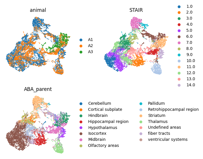
# clustering of spatial embedding
cluster_func(adata, clustering='mclust', use_rep='STAIR', cluster_num=14, key_add='STAIR')

sc.pp.neighbors(adata, use_rep='STAIR')
sc.tl.umap(adata, min_dist=0.2)

from matplotlib.pyplot import rc_context
with rc_context({'figure.figsize': (3,3)}):
    sc.pl.umap(adata, color=['animal', 'STAIR', 'ABA_parent'], frameon=False, ncols=2, show=True)

R[write to console]:                    __           __
   ____ ___  _____/ /_  _______/ /_
  / __ `__ \/ ___/ / / / / ___/ __/
 / / / / / / /__/ / /_/ (__  ) /_
/_/ /_/ /_/\___/_/\__,_/____/\__/   version 6.0.0
Type 'citation("mclust")' for citing this R package in publications.

fitting ...
  |======================================================================| 100%

adata.obs['Domain'] = adata.obs['STAIR'].replace({'1.0':'Layer 1-3', '2.0':'Hippocampus', '3.0':'Olfactory area', '4.0':'Midbrain', '5.0':'Layer 4-5',
                                                  '6.0':'Fiber tracts', '7.0':'Striatum', '8.0':'Cortical subplate', '9.0':'Pallidum', '10.0':'Thalamus',
                                                  '11.0':'Hindbrain', '12.0':'Layer 6', '13.0':'Retrohippocampus', '14.0':'Hypothalamus'})

Reconstruction in z-axis

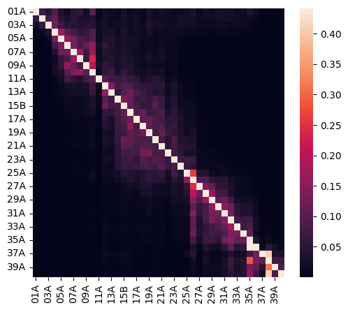
# attention heatmap
import seaborn as sns

vmax = atte[atte!=1].max().max()
vmin = atte[atte!=1].min().min()
plt.figure(figsize=(5.8,5))
sns.heatmap(atte, vmax=vmax, vmin=vmin)
plt.show()
plt.close()

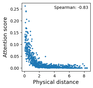
# attention-spatial consistency
from scipy.stats import spearmanr

use = adata.obs[['section_index', 'stereo_AP']].drop_duplicates()
use.index = use['section_index']
use = use['stereo_AP']

attes = []
dists = []
for i in keys_use:
    for j in keys_use:
        if (i != j) & (i < j):
            atte_tmp = (atte.loc[i,j] + atte.loc[j,i]) / 2
            dist_tmp = abs(use[i] - use[j])
            attes.append(atte_tmp)
            dists.append(dist_tmp)


plt.figure(figsize=(3,3))
plt.scatter(dists, attes, s=5)
plt.xlabel('Physical distance', fontsize=13)
plt.ylabel('Attention score', fontsize=13)
plt.text(4, 0.25, 'Spearman: ' + str(round(spearmanr(attes, dists)[0], 2)))
# plt.savefig(f'./{result_path}/atte-dist.pdf', bbox_inches='tight')
plt.show()
plt.close()

dists = sort_slices(atte, start='40A')
dists

{'40A': 0.0,
 '38B': 0.760415375,
 '39A': 0.04691155749999998,
 '35A': 1.610285013,
 '37A': 1.4979991725000001,
 '32A': 2.4965745779999997,
 '34A': 2.492195527,
 '36B': 0.851979199,
 '31A': 3.3616935329999995,
 '33A': 1.6244032879999997,
 '30A': 4.218250467999999,
 '29A': 5.086691825999999,
 '28A': 5.919059945999999,
 '26B': 6.771626910999999,
 '25A': 7.5651357809999995,
 '27A': 5.939053285999999,
 '23A': 8.495861136,
 '20B': 9.4064170935,
 '15B': 10.2982179735,
 '16A': 9.4061976985,
 '18A': 8.5420226585,
 '17A': 8.515853118499999,
 '19A': 7.6612188835,
 '21A': 6.7631627535000005,
 '22A': 6.759656231,
 '24A': 5.839298239500001,
 '12A': 11.191926668499999,
 '14A': 11.189227366499999,
 '11A': 12.131396181,
 '13A': 10.346695593499998,
 '10B': 11.281462848999999,
 '08A': 12.082449793999999,
 '09A': 12.1278575415,
 '06A': 12.988991791499998,
 '07A': 12.911634198999998,
 '05A': 13.848461131499999,
 '04A': 14.693740771499998,
 '03A': 15.613696377999998,
 '02A': 16.538712912999998,
 '01A': 17.470906248}

adata.obs['z_rec'] = adata.obs['section_index'].replace(dists).astype(float)
adata.obs['z_rec'] = (adata.obs['z_rec']- adata.obs['z_rec'].min()) / (adata.obs['z_rec'].max() - adata.obs['z_rec'].min())

z_max, z_min = adata.obs['stereo_AP'].max(), adata.obs['stereo_AP'].min()
adata.obs['z_rec'] = adata.obs['z_rec'] * (z_max - z_min) + z_min
adata.obs['z_rec']
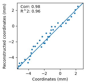
data = adata.obs[['stereo_AP', 'z_rec']].drop_duplicates()

from scipy.stats import pearsonr
from sklearn.metrics import r2_score
import matplotlib.pyplot as plt
import numpy as np

vmin = np.array(data['z_rec'].tolist() + data['stereo_AP'].tolist()).min()
vmax = np.array(data['z_rec'].tolist() + data['stereo_AP'].tolist()).max()

plt.figure(figsize=(3,3))
plt.plot([vmin, vmax],[vmin, vmax])
plt.scatter(data['stereo_AP'], data['z_rec'], s=8)
plt.text(-5,1.7,'Corr: ' + str(pearsonr(data['stereo_AP'], data['z_rec'])[0].round(2)) + '\n' + \
         "R^2: " + str(r2_score(data['stereo_AP'], data['z_rec']).round(2))
         )
plt.xlim([vmin, vmax])
plt.ylim([vmin, vmax])
plt.xlabel('Coordinates (mm)')
plt.ylabel('Reconstructed coordinates (mm)')
# plt.savefig(f'loca_part.png', bbox_inches='tight', dpi=300)
plt.show()
plt.close()

Spatial location alignment in x-axis and y-axis

adata.obs[['section_index', 'z_rec']].drop_duplicates()
slice_order = adata.obs[['section_index', 'z_rec']].drop_duplicates().sort_values('z_rec', ascending=False)['section_index'].tolist()

loc_align = Loc_Align(adata, batch_key='section_index', batch_order=keys_use, result_path=result_path)

anchors = loc_align.init_align( emb_key = 'STAIR',
                                spatial_key = 'spatial',
                                num_mnn = 1,
                                return_result = True)

loc_align.detect_fine_points(  domain_key = 'ABA_parent',
                               slice_boundary = True,
                               domain_boundary = True,
                               num_domains = 1,
                               alpha = 500,
                               return_result = False)

loc_align.plot_edge(spatial_key = 'transform_init',
                    figsize = (6,6),
                    s=2)

adata = loc_align.fine_align()

Performing initial alignment of the 1 pair of data...
Finding similar pairs using STAIR...
Aligning slices using 17 pairs of similar spots!
Performing initial alignment of the 2 pair of data...
Finding similar pairs using STAIR...
Aligning slices using 57 pairs of similar spots!
Performing initial alignment of the 3 pair of data...
Finding similar pairs using STAIR...
Aligning slices using 70 pairs of similar spots!
Performing initial alignment of the 4 pair of data...
Finding similar pairs using STAIR...
Aligning slices using 77 pairs of similar spots!
Performing initial alignment of the 5 pair of data...
Finding similar pairs using STAIR...
Aligning slices using 98 pairs of similar spots!
Performing initial alignment of the 6 pair of data...
Finding similar pairs using STAIR...
Aligning slices using 120 pairs of similar spots!
Performing initial alignment of the 7 pair of data...
Finding similar pairs using STAIR...
Aligning slices using 135 pairs of similar spots!
Performing initial alignment of the 8 pair of data...
Finding similar pairs using STAIR...
Aligning slices using 92 pairs of similar spots!
Performing initial alignment of the 9 pair of data...
Finding similar pairs using STAIR...
Aligning slices using 123 pairs of similar spots!
Performing initial alignment of the 10 pair of data...
Finding similar pairs using STAIR...
Aligning slices using 77 pairs of similar spots!
Performing initial alignment of the 11 pair of data...
Finding similar pairs using STAIR...
Aligning slices using 90 pairs of similar spots!
Performing initial alignment of the 12 pair of data...
Finding similar pairs using STAIR...
Aligning slices using 165 pairs of similar spots!
Performing initial alignment of the 13 pair of data...
Finding similar pairs using STAIR...
Aligning slices using 119 pairs of similar spots!
Performing initial alignment of the 14 pair of data...
Finding similar pairs using STAIR...
Aligning slices using 182 pairs of similar spots!
Performing initial alignment of the 15 pair of data...
Finding similar pairs using STAIR...
Aligning slices using 168 pairs of similar spots!
Performing initial alignment of the 16 pair of data...
Finding similar pairs using STAIR...
Aligning slices using 199 pairs of similar spots!
Performing initial alignment of the 17 pair of data...
Finding similar pairs using STAIR...
Aligning slices using 196 pairs of similar spots!
Performing initial alignment of the 18 pair of data...
Finding similar pairs using STAIR...
Aligning slices using 219 pairs of similar spots!
Performing initial alignment of the 19 pair of data...
Finding similar pairs using STAIR...
Aligning slices using 145 pairs of similar spots!
Performing initial alignment of the 20 pair of data...
Finding similar pairs using STAIR...
Aligning slices using 170 pairs of similar spots!
Performing initial alignment of the 21 pair of data...
Finding similar pairs using STAIR...
Aligning slices using 196 pairs of similar spots!
Performing initial alignment of the 22 pair of data...
Finding similar pairs using STAIR...
Aligning slices using 170 pairs of similar spots!
Performing initial alignment of the 23 pair of data...
Finding similar pairs using STAIR...
Aligning slices using 167 pairs of similar spots!
Performing initial alignment of the 24 pair of data...
Finding similar pairs using STAIR...
Aligning slices using 110 pairs of similar spots!
Performing initial alignment of the 25 pair of data...
Finding similar pairs using STAIR...
Aligning slices using 137 pairs of similar spots!
Performing initial alignment of the 26 pair of data...
Finding similar pairs using STAIR...
Aligning slices using 128 pairs of similar spots!
Performing initial alignment of the 27 pair of data...
Finding similar pairs using STAIR...
Aligning slices using 130 pairs of similar spots!
Performing initial alignment of the 28 pair of data...
Finding similar pairs using STAIR...
Aligning slices using 143 pairs of similar spots!
Performing initial alignment of the 29 pair of data...
Finding similar pairs using STAIR...
Aligning slices using 122 pairs of similar spots!
Performing initial alignment of the 30 pair of data...
Finding similar pairs using STAIR...
Aligning slices using 200 pairs of similar spots!
Performing initial alignment of the 31 pair of data...
Finding similar pairs using STAIR...
Aligning slices using 114 pairs of similar spots!
Performing initial alignment of the 32 pair of data...
Finding similar pairs using STAIR...
Aligning slices using 94 pairs of similar spots!
Performing initial alignment of the 33 pair of data...
Finding similar pairs using STAIR...
Aligning slices using 119 pairs of similar spots!
Performing initial alignment of the 34 pair of data...
Finding similar pairs using STAIR...
Aligning slices using 94 pairs of similar spots!
Performing initial alignment of the 35 pair of data...
Finding similar pairs using STAIR...
Aligning slices using 51 pairs of similar spots!
Performing initial alignment of the 36 pair of data...
Finding similar pairs using STAIR...
Aligning slices using 34 pairs of similar spots!
Performing initial alignment of the 37 pair of data...
Finding similar pairs using STAIR...
Aligning slices using 47 pairs of similar spots!
Performing initial alignment of the 38 pair of data...
Finding similar pairs using STAIR...
Aligning slices using 51 pairs of similar spots!
Performing initial alignment of the 39 pair of data...
Finding similar pairs using STAIR...
Aligning slices using 56 pairs of similar spots!
Performing fine alignment of the 1 pair of data...
Performing fine alignment of the 2 pair of data...
Performing fine alignment of the 3 pair of data...
Performing fine alignment of the 4 pair of data...
Performing fine alignment of the 5 pair of data...
Performing fine alignment of the 6 pair of data...
Performing fine alignment of the 7 pair of data...
Performing fine alignment of the 8 pair of data...
Performing fine alignment of the 9 pair of data...
Performing fine alignment of the 10 pair of data...
Performing fine alignment of the 11 pair of data...
Performing fine alignment of the 12 pair of data...
Performing fine alignment of the 13 pair of data...
Performing fine alignment of the 14 pair of data...
Performing fine alignment of the 15 pair of data...
Performing fine alignment of the 16 pair of data...
Performing fine alignment of the 17 pair of data...
Performing fine alignment of the 18 pair of data...
Performing fine alignment of the 19 pair of data...
Performing fine alignment of the 20 pair of data...
Performing fine alignment of the 21 pair of data...
Performing fine alignment of the 22 pair of data...
Performing fine alignment of the 23 pair of data...
Performing fine alignment of the 24 pair of data...
Performing fine alignment of the 25 pair of data...
Performing fine alignment of the 26 pair of data...
Performing fine alignment of the 27 pair of data...
Performing fine alignment of the 28 pair of data...
Performing fine alignment of the 29 pair of data...
Performing fine alignment of the 30 pair of data...
Performing fine alignment of the 31 pair of data...
Performing fine alignment of the 32 pair of data...
Performing fine alignment of the 33 pair of data...
Performing fine alignment of the 34 pair of data...
Performing fine alignment of the 35 pair of data...
Performing fine alignment of the 36 pair of data...
Performing fine alignment of the 37 pair of data...
Performing fine alignment of the 38 pair of data...
Performing fine alignment of the 39 pair of data...

3D Visualization

import plotly.express as px
import matplotlib

hex_colors = [plt.matplotlib.colors.rgb2hex(color) for color in plt.cm.tab20.colors]

### domain all
adata.obs['Domain'] = adata.obs['Domain'].cat.set_categories(['Midbrain', 'Layer 4-5', 'Thalamus',  'Layer 6',
                                                             'Hypothalamus', 'Layer 1-3',  'Hindbrain',
                                                             'Olfactory area', 'Hippocampus', 'Pallidum', 'Retrohippocampus', 'Striatum',
                                                             'Cortical subplate', 'Fiber tracts'])
domains = adata.obs['Domain'].cat.categories.tolist()
df = adata.obs
fig = px.scatter_3d(df,
                    x='x_pred',
                    y='y_pred',
                    z='z_pred',
                    color='Domain',
                    opacity=1,
                    color_discrete_map={domains[i]:matplotlib.colors.to_hex(plt.cm.get_cmap('tab20')(i)) for i in range(len(domains))},
                    )
fig.update_traces(marker_size = 3)
fig.update_layout(
    height=1000,
    width=1000,
    scene=dict(
        aspectratio=dict(x=1.1, y=1, z=1.3) #改变画布空间比例为1：1：1
        ),
    margin=dict(r=0, l=0, b=0, t=0))
fig

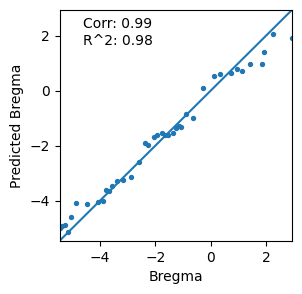
Prediction in z-axis

In addition, we assessed the ability for predicting the z-axis of new slices by STAIR. By sequentially masking the known z-axis coordinates of slices, we predicted the masked value based on attention scores.

# location prediction

preds = []

for query_tmp in keys_use:
    pred_tmp, loc_knowns = loc_predict_z(   adata,
                                            atte,
                                            querys = [query_tmp],
                                            loc_key = 'stereo_AP',
                                            batch_key = 'section_index',
                                            knowns = None,
                                            num_mnn = 10)
    preds.append(pred_tmp[0])


from scipy.stats import pearsonr
from sklearn.metrics import r2_score

use = adata.obs[['section_index', 'stereo_AP']].drop_duplicates()
use.index = use['section_index']
use['pred'] = preds

trues = use['stereo_AP'].tolist()
vmin = np.array(preds + trues).min()
vmax = np.array(preds + trues).max()

plt.figure(figsize=(3,3))
plt.scatter(use['stereo_AP'], use['pred'], s=8)
plt.plot([vmin, vmax],[vmin, vmax])
plt.xlim([vmin, vmax])
plt.ylim([vmin, vmax])
plt.text(vmin+0.1*(vmax-vmin), vmax-0.15*(vmax-vmin),
         'Corr: ' + str(pearsonr(use['stereo_AP'], use['pred'])[0].round(2)) + '\n' + \
         "R^2: " + str(r2_score(use['stereo_AP'], use['pred']).round(2))
         )
plt.xlabel('Bregma')
plt.ylabel('Predicted Bregma')
# plt.savefig(f'./{result_path}/loc_pred.pdf', bbox_inches='tight')
plt.show()
plt.close()

Save

adata.write(f'{result_path}/adata.h5ad')